Abstract
This experiment combined Landsat 8 temperature with Sentinel-2A optical indices to estimate land surface temperature (LST) on a 10 m grid and compared its spatial patterns with HOTSAT-1 supplied SBT imagery acquired on a different date. Temperature was retrieved from Landsat data acquired on 16 October 2023 using NDVI-based emissivity and atmospheric auxiliary variables. Same-day Sentinel-2 reflectance was harmonized empirically for the scene, followed by regression using NDVI, NDBI and Green–NIR NDWI. The initial result, with recalculated 30 m residuals distributed through a smooth correction field, achieved Pearson r=0.841 over 174,927 common land cells, compared with 0.794 for the original Landsat baseline. Local correlation after removing the surrounding 310 m mean also increased from 0.557 to 0.677, whereas recall of the hottest 10% of HOTSAT cells changed only slightly, from 48.2% to 48.6%. Retraining over the full common area produced lower scores than the initial result, and a temperature-rank reversal between a sports field and adjacent bare ground was identified. Spectral differences and reflected sunlight may affect hot-area rank comparisons in the daytime HOTSAT observation, interpreted here as acquired with the night filter. Despite these constraints, improved spatial correlation and local contrast support the usefulness of this approach for exploring relative thermal structure in greater detail. Quantitative validation of individual 10 m temperatures and small hotspots could be strengthened with future HOTSAT day-filter or high-resolution long-wave infrared observations.
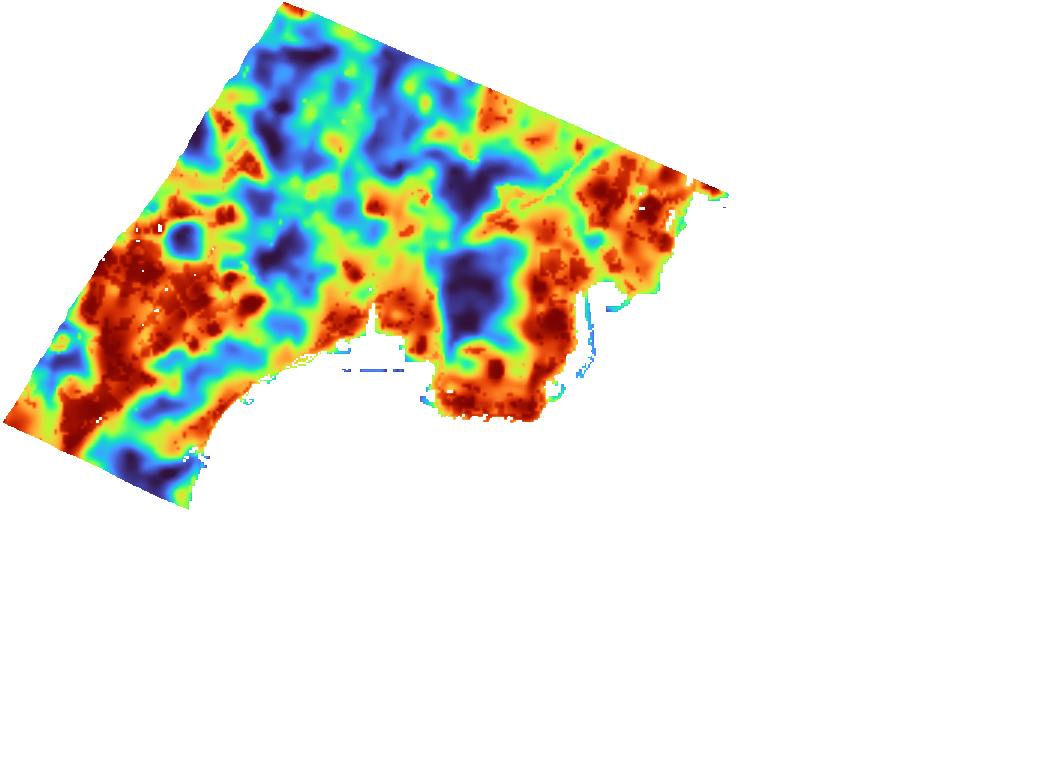 N
N↑1 km
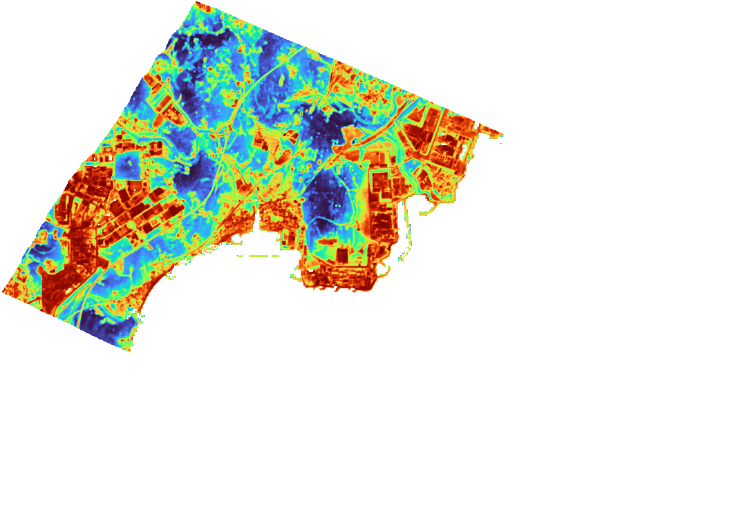 N
N↑1 km
Image temporarily withheld
Background and objectives
Landsat temperature grids and high-resolution optical imagery describe the same surface at different spatial scales. Optical-index-based downscaling learns relationships between coarse-scale temperature and land-cover indices, then applies them to finer-scale optical indices. This experiment used the Landsat–Sentinel-2 index-regression framework of Onačillová et al. (2022) as its starting point.[1] Temperature retrieval, scene-specific reflectance harmonization and residual distribution were adapted to the present workflow, so this is not a complete reproduction of the original study.
The objectives were to assess how closely the additional detail inferred from optical indices matches the spatial structure of a separate thermal observation, and to examine whether temperature ordering over individual surfaces can be distorted even when overall spatial correlation improves. The comparison was limited to the valid HOTSAT footprint around Gori and Gijang.
Data and methods
2.1 Observations and comparison grid
| Data | Acquisition time (KST) | Role |
|---|---|---|
| Landsat 8 | 2023.10.16 10:59:39 | L2 optical/atmospheric auxiliary data and temperature retrieval |
| Sentinel-2A | 2023.10.16 11:17:36.86 | L2A optical indices · 10 m prediction |
| HOTSAT-1 | 2023.10.26 14:23:00 | Supplied SBT · final spatial-pattern comparison |
Landsat and Sentinel were acquired approximately 18 minutes apart. HOTSAT was acquired 10 days after Landsat and approximately 3 hours 23 minutes later in local time. HOTSAT imagery was not used for training, band harmonization, temperature-bias correction or residual calculation.
The comparison grid uses EPSG:32652 with 1,059×768 cells at 10 m spacing and an upper-left origin of (521,835 m, 3,912,585 m). It is aligned by subdividing the Landsat 30 m grid into 3×3 cells. Initial processing used a working area extending 5 km beyond the comparison footprint, then cropped the output. The original Landsat temperature bilinearly interpolated to 10 m served as the downscaling baseline.
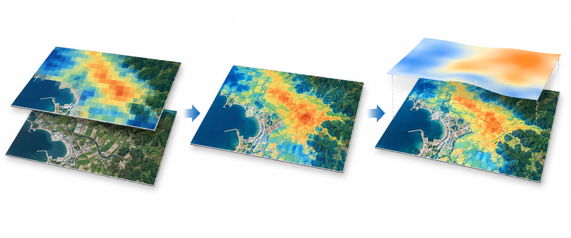
Harmonize Sentinel reflectance
10 m regression prediction P₁₀
Final T₁₀ = P₁₀ + Bz*
2.2 Landsat temperature retrieval
Landsat Collection 2 surface reflectance was converted using SR = DN × 0.0000275 − 0.2. Landsat RED and NIR were used to calculate NDVI and vegetation fraction Pᵥ = clip[(NDVI−0.2)/0.3, 0, 1]², followed by emissivity assigned by NDVI interval. The coefficient choices draw on Yu et al. (2014) and Sekertekin and Bonafoni (2020); the preserved lst_ndvi_model.py defines the actual implementation.[2][3]
| Condition | Emissivity |
|---|---|
| NDVI < 0.2 | 0.973 − 0.047 × RED |
| 0.2 ≤ NDVI ≤ 0.5 | 0.9863 Pᵥ + 0.9668 (1−Pᵥ) + C |
| NDVI > 0.5 | 0.9863 |
| QA_PIXEL water | 0.991 · takes precedence over other branches |
C = (1−0.9668) × 0.9863 × 0.55 × (1−Pᵥ), where RED is surface reflectance. Water was identified using QA information, not negative NDVI alone. The water-emissivity value follows Wang et al. (2019).[4]
Radiance and transmittance were recovered by applying 0.001 to ST_TRAD, ST_URAD and ST_DRAD, and 0.0001 to ST_ATRAN. Landsat 8 MTL constants K₁=774.8853 and K₂=1321.0789 were used. The supplied ASTER-based emissivity was not used as the primary input. The retrieved temperature's 30 m grid spacing is distinct from the thermal sensor's independent observational resolution.
2.3 Reflectance harmonization and temperature regression
Sentinel reflectance was averaged onto the Landsat 30 m grid, then bandwise linear regressions SRL8,b = aᵦ + bᵦ · SRS2,b were fitted. These coefficients were applied to Sentinel 10 m reflectance before calculating indices. The Sentinel metadata BOA offset of −1,000 and quantification factor of 10,000 were included. This is scene-specific empirical harmonization, not a full implementation of official HLS spectral-response and BRDF normalization.
| Index | Definition | Sentinel bands |
|---|---|---|
| NDVI | (NIR−RED)/(NIR+RED) | B08, B04 · both 10 m |
| NDBI | (SWIR1−NIR)/(SWIR1+NIR) | B11 · native 20 m → 10 m, B08 |
| NDWI | (GREEN−NIR)/(GREEN+NIR) | B03, B08 · Green–NIR formulation |
B11 was bilinearly resampled to 10 m; the SWIR input therefore does not contain independent native 10 m spatial information. BLUE is included in reflectance and RGB outputs but does not directly enter these three index equations.
The initial regression used 182,617 clear-land 30 m cells in the surrounding subset. Full-area retraining re-estimated both band harmonization and temperature regression using 7,334,111 30 m cells in the same-day Landsat–Sentinel common area. Both experiments were evaluated over the same HOTSAT comparison area.
2.4 Recalculating and smoothly distributing 30 m residuals
Residuals were calculated as the difference between Landsat temperature and the 10 m regression prediction averaged back to 30 m. The correction field was regularized to discourage large changes between adjacent control points.
E is the set of neighboring control-grid pairs. B bilinearly distributes the control-grid correction z to 10 m, and W gives weight 1 to 30 m blocks with all 3×3 child cells valid, and 0 to incomplete blocks. Smoothing was applied to the residual correction field to be added, not to the optical prediction image. This optimization does not enforce exact agreement with 30 m averages. It is a custom modification distinct from the original paper's residual resampling and smoothing.
2.5 HOTSAT aggregation and evaluation definitions
Spatial averaging used the actual overlap areas between native HOTSAT SBT cells of approximately 5.713 m and target 10 m cells as weights. This averages the supplied SBT values; it does not average radiance after an inverse temperature conversion. A valid UDM value of 0 was not treated as missing. Finite values flagged for saturation were retained, with separate QA preserved. Comparison statistics used only the common valid area in which source data fully covered each target cell.
| Subset | Condition / cell count |
|---|---|
| Full common valid area | 430,192 cells at 10 m · complete coverage |
| Primary evaluation: land | SCL 4·5, excluding Landsat water · 174,927 cells |
| Local contrast | Subtract 31×31-cell (310×310 m) mean · 149,389 cells |
| Local-contrast support | Valid neighborhood support and land fraction each ≥90% |
| Aggregation to 30, 60 and 100 m | Common valid area and land fraction per block each ≥90% |
Evaluation metrics were land Pearson r, Spearman ρ, Pearson r of local contrast, and recall of the hottest 10%. Recall was defined as the proportion of the hottest 10% of HOTSAT land cells also falling within the hottest 10% of the comparison image. Because cells are spatially autocorrelated, cell counts were not treated as independent sample sizes, and no p-values or confidence intervals based on those counts were reported.
Results
3.1 Spatial patterns of the initial downscaling
| Result | Land r | Rank ρ | Local r | Top-10% recall |
|---|---|---|---|---|
| Original Landsat · bilinear 10 m | 0.794 | 0.809 | 0.557 | 48.2% |
| Initial regression · no residual | 0.802 | 0.827 | 0.661 | 35.0% |
| Initial regression · smooth residual | 0.841 | 0.858 | 0.677 | 48.6% |
Land n=174,927 cells; local contrast n=149,389 cells. Recall uses the hottest 10% of the original temperature distributions, not local deviations.
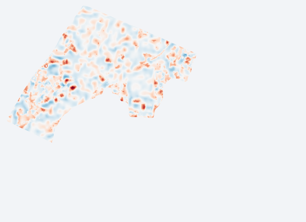
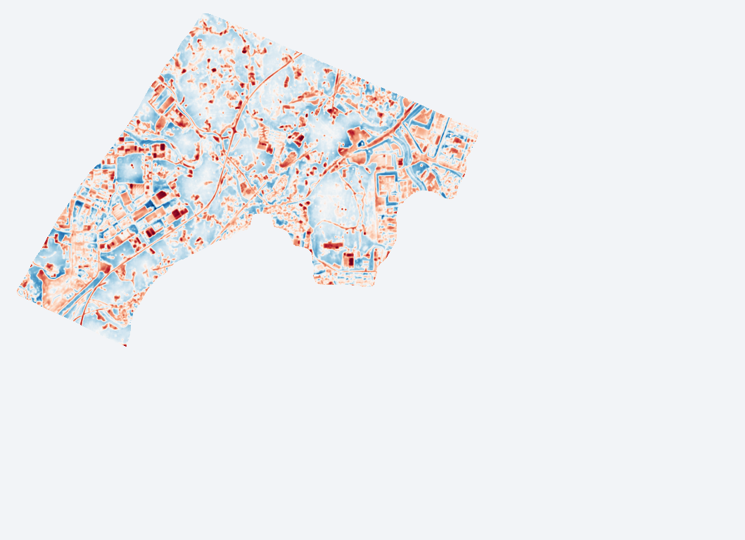
Without residual correction, land correlation was 0.802, slightly above the 0.794 baseline, while local correlation increased from 0.557 to 0.661. Adding the smooth residual gave the highest values for both metrics: 0.841 and 0.677. In contrast, top-10% recall improved by only approximately 0.4 percentage points, from 48.2% at baseline to 48.6% in the final result. The image without residual correction depicted local structure but had lower recall, at 35.0%; visual detail and hot-area recovery did not improve in parallel.
Image temporarily withheld
N↑2 km
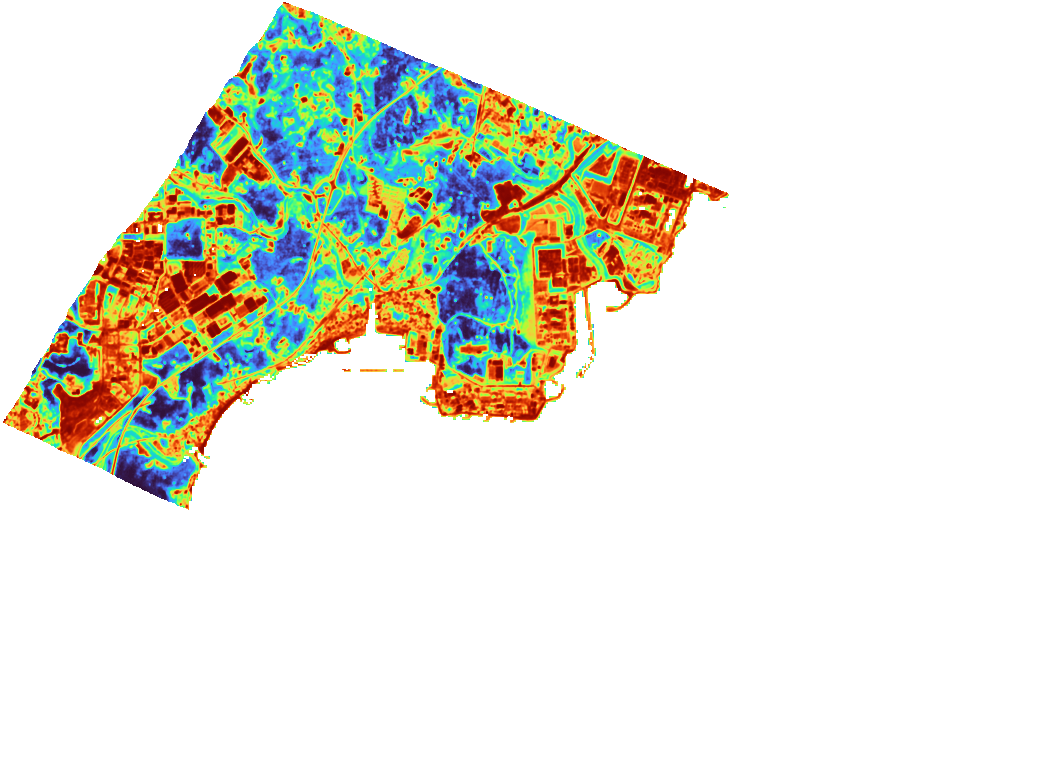 N
N↑2 km
N↑2 km
Source: native-grid PNGs in comparison_20231016_20231026/visuals · 1,059×768 cells at 10 m · grid north up.
3.2 Local contrast and reaggregation consistency
After removing the surrounding 310 m mean, correlation for the initial corrected result remained higher than the baseline. This metric helps distinguish agreement from that explained only by broad thermal gradients. Land correlations after averaging over identical spatial blocks were 0.828 at baseline and 0.868 after correction at 30 m; 0.875 and 0.902 at 60 m; and 0.914 and 0.927 at 100 m. Correlation at coarser block sizes was not translated into 10 m temperature accuracy.
Image temporarily withheld
 N
N↑2 km
 N
N↑2 km
Source: assets/local_0·1·3.png from the earlier report · numerical source: LOCAL_CONTRAST_310m_10m.tif.
Across 19,325 complete 30 m blocks within the HOTSAT footprint, the RMS difference between predictions reaggregated to 30 m and the original Landsat temperature decreased from 1.842°C without residual correction to 0.963°C after correction. This indicates improved internal consistency with the Landsat background temperature, not error against independent observational ground truth.
3.3 Retraining over the full common area
Although the training sample increased from 182,617 to 7,334,111 cells, scores were lower than those of the initial corrected result. There were no differences in the evaluation-area validity masks. Of the full training sample, 75.4% had NDVI≥0.6: a larger sample did not imply balanced representation of land-cover types.
| Result | Land r | Rank ρ | Local r | Top-10% recall |
|---|---|---|---|---|
| Initial · no residual | 0.802 | 0.827 | 0.661 | 35.0% |
| Full area · no residual | 0.780 | 0.806 | 0.628 | 32.4% |
| Initial · smooth residual | 0.841 | 0.858 | 0.677 | 48.6% |
| Full area · smooth residual | 0.824 | 0.843 | 0.641 | 44.8% |
Source: full_scene_20231016/paired_comparison.json · identical land mask. The SVG charts were constructed from the original numerical results.
The initial temperature-regression coefficients [β₀, β₁, β₂, β₃] were [31.0071, −7.1295, 2.4962, 2.6248], compared with [30.0669, −18.2404, −0.4286, −8.1665] for the full area. Because band harmonization and temperature regression changed together, the decline in scores cannot be attributed independently to either stage.
3.4 Temperature ordering of a sports field and adjacent bare ground
A green surface shaped like a sports field (A) and bare ground to its east (B) were compared using 30 m×30 m windows. In the initial corrected result, A became cooler than B, reversing their ordering in the original Landsat image. Surface materials, including whether the field was artificial turf, were not confirmed.
Image temporarily withheld
 N
N↑100 mAB
Source: assets/target_13_hot·smooth.png from the earlier report · A (525550, 3910500), B (525660, 3910500), EPSG:32652.
| Image | A (°C) | B (°C) | A−B (°C) |
|---|---|---|---|
| HOTSAT SBT | 41.2556 | 33.9725 | +7.28 |
| Original Landsat | 30.5463 | 29.4906 | +1.06 |
| Initial · no residual | 26.0989 | 28.8649 | -2.77 |
| Initial · smooth residual | 28.9975 | 30.6589 | -1.66 |
For the central 10 m cell of the sports field, Sentinel NDVI changed from 0.271 before harmonization to 0.504 afterward. This suggests a possible influence from regression predicting lower, vegetation-like temperatures. However, inter-sensor reflectance differences, the regression, emissivity assumptions and differing thermal observation conditions may all contribute; this was not established as the cause of the rank reversal.
3.5 Follow-up close-up comparison around Gori
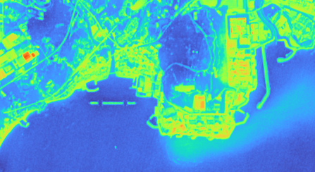
Full-common-area retraining results and a later HOTSAT rendering with QA exclusions disabled were enlarged over the same extent. This figure visually compares forest, facility and coastal boundaries and local thermal structure. Its processing version is distinguished from that used in the preceding quantitative tables for the initial experiment.
 N
N↑1 km
Image temporarily withheld
Source: two native-crop PNGs in closeup_Kori_reference_area. Original temperatures and display colours were not changed.
The images share the coastline and broad arrangement of forest and facilities, but HOTSAT shows more localized warm features along some facility boundaries. These differences can help identify surfaces for further investigation. Because colour ranges and observation conditions differ, this visual comparison alone was not used to rank hot-feature intensity or 10 m temperature accuracy.
Discussion and limitations
4.1 Improved spatial patterns and independent thermal information
The initial results showed higher correlation with HOTSAT land spatial patterns when fine optical-index structure was combined with Landsat background temperature. Yet hot-area recall changed little and the ordering of individual surfaces was distorted. Boundaries appearing on the 10 m grid should therefore not be interpreted as boundaries from new independent thermal observations. The 30 m reaggregation RMS after residual correction likewise measures consistency with the input Landsat data.
4.2 Dual use of NDVI and emissivity assumptions
NDVI serves two different roles in this experiment: first, estimating emissivity to convert thermal radiance to temperature; and second, explaining the spatial variation of that temperature as a regression predictor. This is not computationally contradictory, but the training target already contains an NDVI dependence. Part of the temperature–NDVI relationship may therefore reflect assumptions in the emissivity model alongside actual surface thermal properties. A strong regression fit alone does not establish that NDVI supplies independent thermal information.
Onačillová et al. (2022) also discussed the influence of NDVI-classified emissivity when interpreting scatterplots in their case study, then used NDVI, NDBI and NDWI in LST regression (§3.1, Figure 5). Their separately described GEE implementation (§2.4) and public code read Collection 2 Level 2 ST_B10 as the temperature input.[1] This differs from directly retrieving temperature again using NDVI-threshold emissivity, as done here. The official ST product also uses auxiliary information including ASTER emissivity and NDVI, so it is not a target entirely independent of optical information.[8] A procedure explicitly separating and testing the two stages of NDVI dependence was not found in the paper or the public code examined.
Accordingly, these results are interpreted as performance of a temperature-retrieval and downscaling system that incorporates optical information. Comparing outputs with different emissivity assumptions for the same thermal radiance, alongside regressions excluding NDVI, could help distinguish its two roles. Those experiments were not performed in this report.
4.3 NIR harmonization and generalization across surfaces
In a separate NIR diagnostic, Sentinel B08–Landsat B5 correlation was 0.422, B8A–Landsat B5 correlation was 0.418, and B08–B8A correlation was 0.988. Switching to B8A did not resolve the low scene-wide NIR correlation, so the broader B08 spectral band alone cannot explain the issue. This diagnostic was not a rerun that changed the existing downscaled outputs.
At the sports-field location, viewing zenith angles were approximately 1.44° for Landsat B5 and 1.03° for Sentinel B08, both near nadir. This does not support strongly oblique viewing at that point as the primary explanation. It also does not isolate azimuth, solar angle, BRDF, terrain illumination, atmospheric correction or fine-scale registration effects. The large NIR regression intercept and the change in field NDVI remain diagnostic clues.
4.4 Comparison observations and reflected signals
HOTSAT and Landsat differ by 10 days in acquisition date, as well as in time of day, spectral band and temperature definition. Effects of weather, surface moisture, shadows and facility operations were not removed. HOTSAT supplied SBT and LST retrieved using emissivity and atmospheric information were not treated as a ground-truth/prediction pair of the same physical quantity.
This report interprets the source HOTSAT metadata satvu:filter=night as the night filter actually used for the observation. Current SatVu specifications give 3.70–4.95 μm for night mode and 4.50–4.95 μm for day mode.[9] At shorter MWIR wavelengths during daytime, both surface emission and reflected solar radiation can be detected, and additional reflected radiance can increase brightness temperature.[10] Consequently, spectral differences and reflected sunlight are considered major candidate explanations when interpreting differences between this daytime night-filter image and Landsat LST. The current band specifications support this physical interpretation; the detailed spectral response at the time of acquisition has not been verified.
If reflected contributions are concentrated on particular roofs or surfaces, they can change hot-area rankings and limit top-10% overlap even when broad spatial patterns correlate well. A uniform temperature increase across all cells would preserve ranks; the important factor here is surface-dependent reflected contributions. Top-10% recall is therefore interpreted as hot-area agreement reflecting both downscaling performance and differences in spectral band, temperature definition and acquisition conditions. The small additional improvement from 48.2% for original Landsat to 48.6% after downscaling remains a result, but it alone cannot determine whether fine thermal structure was successfully reconstructed.
HOTSAT hot features concentrated on some roof faces and edges are consistent with the reflection hypothesis, but actual heating, shadows, operational state and viewing geometry are also possible explanations. Solar elevation was 32.49° and off-nadir angle 39.88° for this scene. Reflected contributions were not quantified because surface normals, spectral reflectance, actual filter response and the product's reflection-correction history were unavailable. Saturation QA does not diagnose reflection, so the absence of a saturation flag does not rule it out. Interpreting the filter as night mode is distinct from determining the reflected contribution to an individual hot feature.
In the ±20 m positional-shift sensitivity test, the initial corrected result had its highest correlation at the original coordinates. This is a diagnostic within the tested range, not proof that all local registration errors are absent. Land–water thermal differences contribute to high correlation over the combined land and sea area, so land-only metrics were used as the primary results. Reported cell counts are counts of valid comparison-grid cells, not independent experimental replicates.
Conclusions and next steps
This experiment showed useful results for depicting relative warm/cool distributions and thermal spatial structure in finer detail by combining optical information with Landsat thermal data. Initial downscaling increased land Pearson r from 0.794 to 0.841 and local-contrast correlation after removal of the surrounding 310 m background from 0.557 to 0.677. More clearly expressed boundaries and thermal contrasts around forests, urban areas and facilities visually support the approach's potential alongside these metric improvements.
The current outputs can be used to explore relative thermal environments around cities and facilities and to select areas requiring additional observation or field validation. Representing finer structure while retaining broad temperature distributions offers research and practical value. “Meaningful” here refers to improved spatial patterns and potential utility, not a separate test of statistical significance.
Additional improvement in top-10% recall was small, expanding the training area did not improve performance, and temperature-rank reversals remained for some surfaces. Comparisons between daytime night-filter HOTSAT SBT and Landsat LST can also reflect combined differences in spectral band, temperature definition, reflected signals and acquisition conditions. Current hot-area comparisons therefore have limitations as independent validation of downscaling performance. These limitations do not negate the improved spatial correlation and local contrast or the value of the imagery for visual exploration.
Quantitative assessment of individual facilities' absolute temperatures at 10 m and of small hotspots requires further validation. Future HOTSAT day-filter imagery or high-resolution long-wave infrared (LWIR) imagery comparable to Landsat could strengthen this assessment. Evaluation should minimize acquisition-date and time differences and consistently handle registration, spatial response, emissivity, atmospheric correction and temperature definitions, reducing the influence of spectral differences and reflected signals. Day-filter imagery should not be assumed to be reflection-free ground truth; in-situ temperature observations should support absolute-temperature validation where possible.
Next experiment · TIR-to-TIR super-resolution Not performed
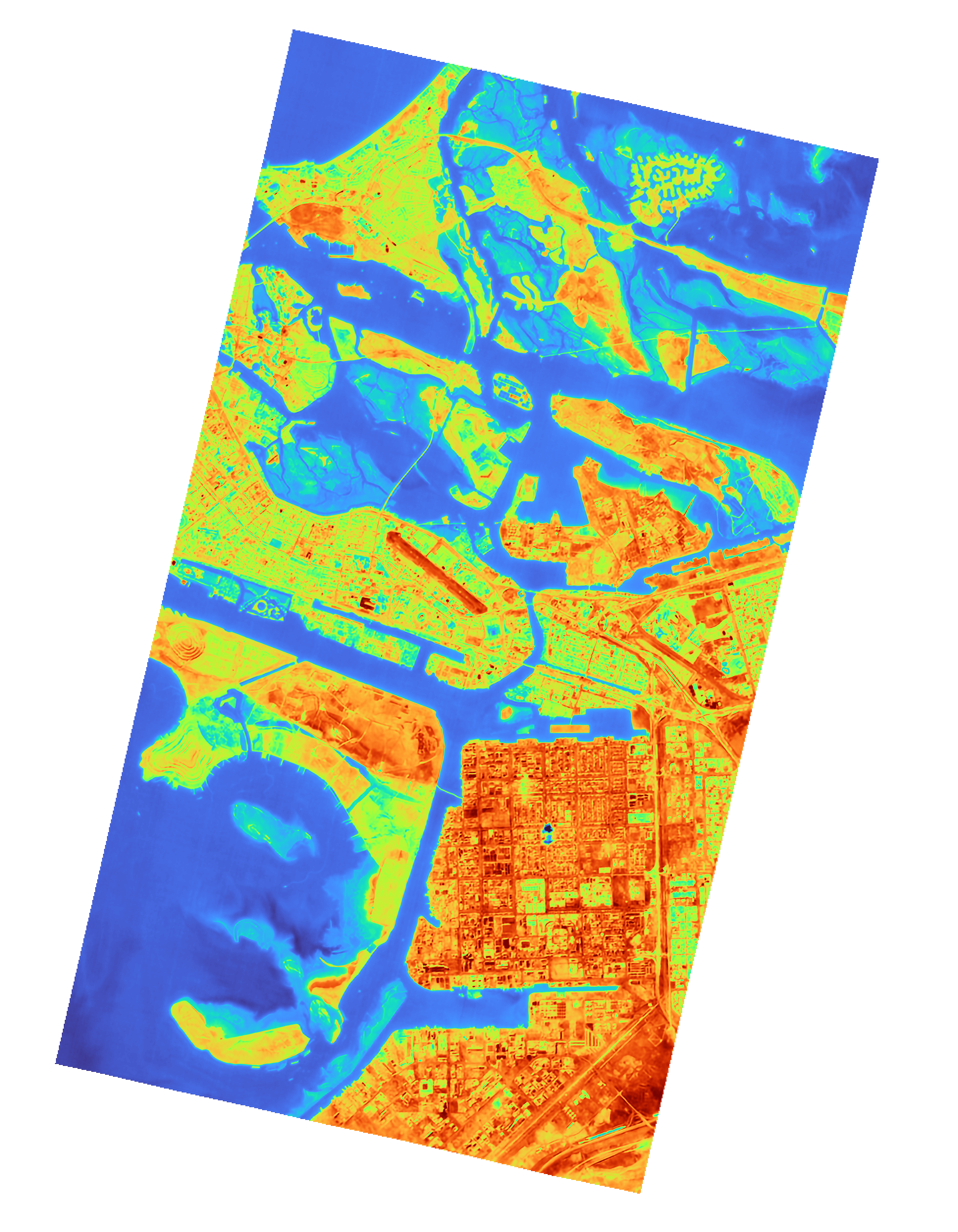
Future work will explore LST-to-LST restoration learned from thermal information alone, informed by public descriptions of Constellr HiVE/SkyBee. The official Sharpening Layer documentation checked in October 2026 specifies an RRDB neural network producing 10 m LST from 30 m LST without auxiliary optical bands.[5] Archived LSTzoom documentation describes degrading airborne high-resolution thermal imagery using sensor PSF and downsampling, learning the inverse transformation, and evaluating on separate airborne scenes.[6]
The proposed follow-up is to construct degradation/restoration experiments that account for Landsat's actual sensor spatial response, then compare temperature error, local contrast and hot-area recovery against the optical-based results on separate scenes. The vendor's detailed code and weights have not been verified, so this is not described as a complete reproduction. Use of RRDB alone does not establish that a GAN or perceptual loss is used.[7] The 10 m product in the existing Abu Dhabi 30 m/10 m open sample will not be treated as independent observational ground truth. No additional downloads or model training were performed for this plan.
 N
N↑500 m
 N
N↑500 m
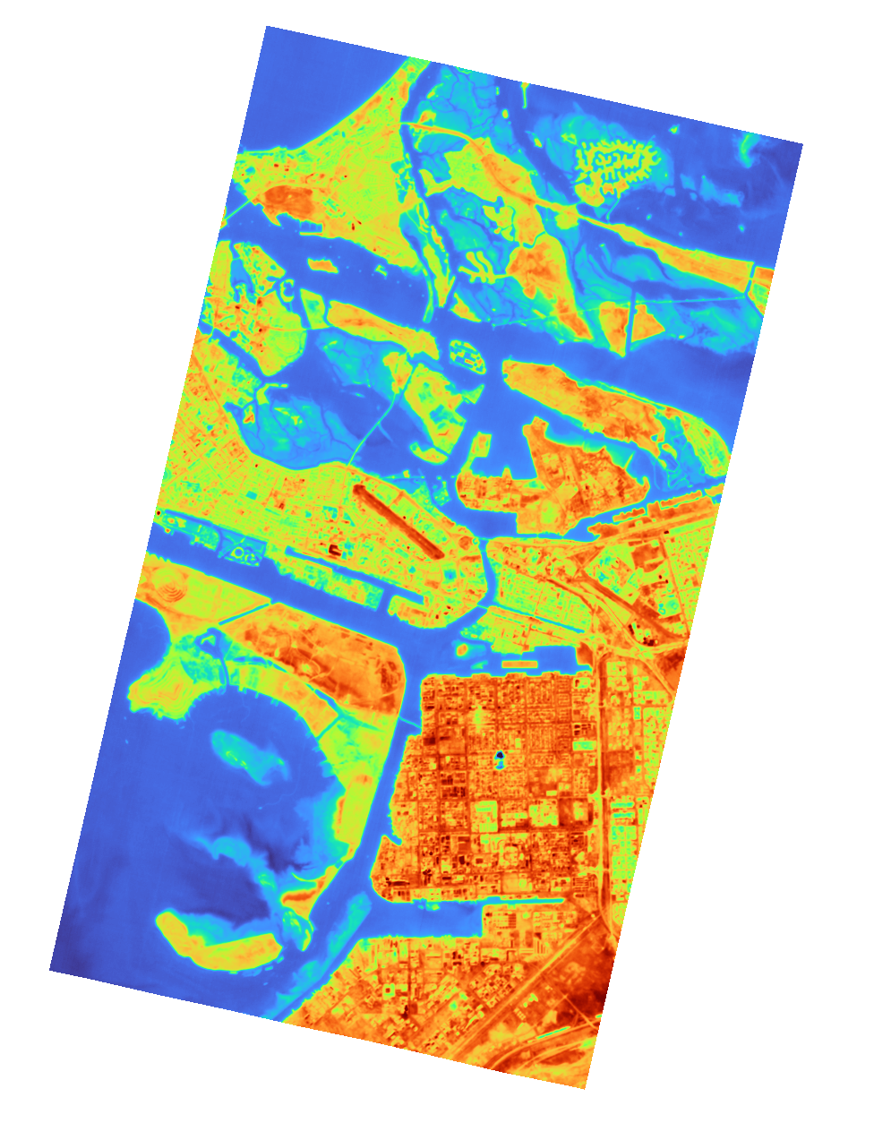
Source: previously archived products from the Constellr Open Data Programme. EPSG:32640; crop extent E 244,200–247,800 m / N 2,693,790–2,697,390 m. Original values, colours and masks are retained; only the displayed extent is narrowed.
Within the close-up, the 10 m product depicts intra-block temperature contrasts and linear boundaries in finer detail than the 30 m image. This area illustrates a visual difference in spatial detail; it is not a validation sample representative of quantitative performance across the full scene. Public metadata alone do not establish the exact model version used. Image sharpness was not equated with improved actual temperature accuracy.
References
- Onačillová, K., Gallay, M., Paluba, D., Péliová, A., Tokarčík, O., & Laubertová, D. (2022). Combining Landsat 8 and Sentinel-2 Data in Google Earth Engine to Derive Higher Resolution Land Surface Temperature Maps in Urban Environment. Remote Sensing, 14(16), 4076. 10.3390/rs14164076. Author code: LST-downscaling-to-10m-GEE · GEE implementation examined (2026.10.08).
- Yu, X., Guo, X., & Wu, Z. (2014). Land Surface Temperature Retrieval from Landsat 8 TIRS—Comparison between Radiative Transfer Equation-Based Method, Split Window Algorithm and Single Channel Method. Remote Sensing, 6(10), 9829–9852. 10.3390/rs6109829.
- Sekertekin, A., & Bonafoni, S. (2020). Land Surface Temperature Retrieval from Landsat 5, 7, and 8 over Rural Areas: Assessment of Different Retrieval Algorithms and Emissivity Models and Toolbox Implementation. Remote Sensing, 12(2), 294. 10.3390/rs12020294.
- Wang, L., Lu, Y., & Yao, Y. (2019). Comparison of Three Algorithms for the Retrieval of Land Surface Temperature from Landsat 8 Images. Sensors, 19(22), 5049. 10.3390/s19225049.
- Constellr. LSTprecision Data Bundle Description — Sharpening Layer. Official product documentation. Page update label: October 2026. Accessed: 2026.10.08. Official Sharpening Layer description.
- Constellr. LSTzoom. Archived product documentation. Page update label: March 2026. Accessed: 2026.10.08. Archived LSTzoom documentation.
- Wang, X., et al. (2018). ESRGAN: Enhanced Super-Resolution Generative Adversarial Networks. arXiv:1809.00219. Background reference for the RRDB architecture. arXiv:1809.00219.
- U.S. Geological Survey. Landsat Collection 2 Surface Temperature. Official product-generation documentation. Accessed: 2026.10.08. Temperature-product inputs and emissivity information.
- SatVu. Imagery Product Spec — Sensor Information. Current MWIR day/night band specifications. Accessed: 2026.10.08. Official imagery product specification.
- CIRA / NOAA. Shortwave IR Window Channel (3.9 micron): Reflected Solar Component. General principles of daytime reflected and emitted radiation. Accessed: 2026.10.08. The reflected component at 3.9 μm.
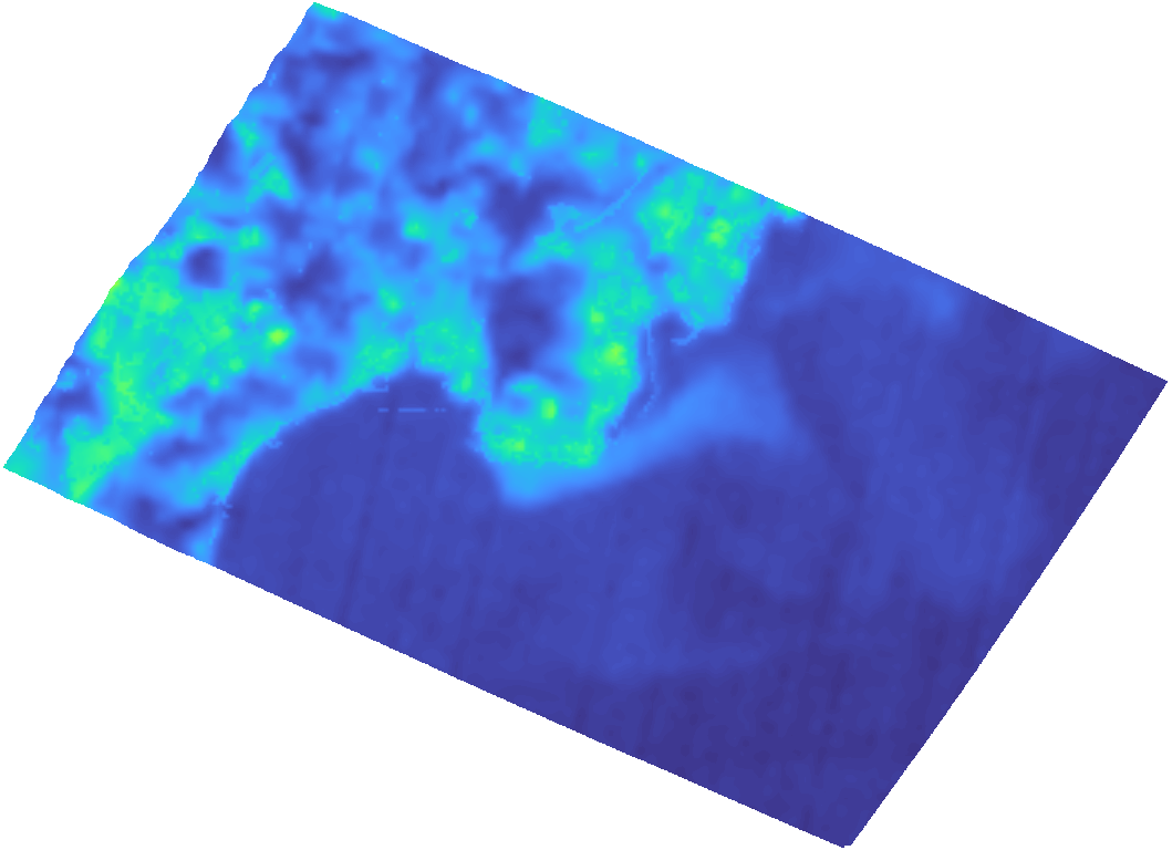
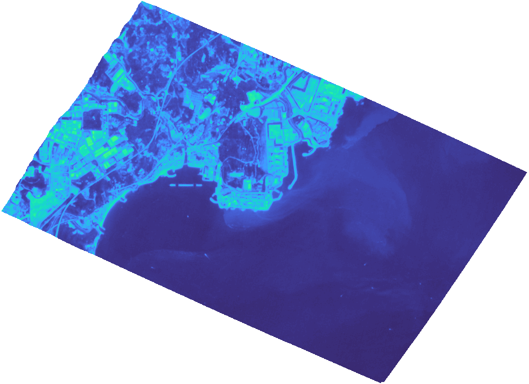
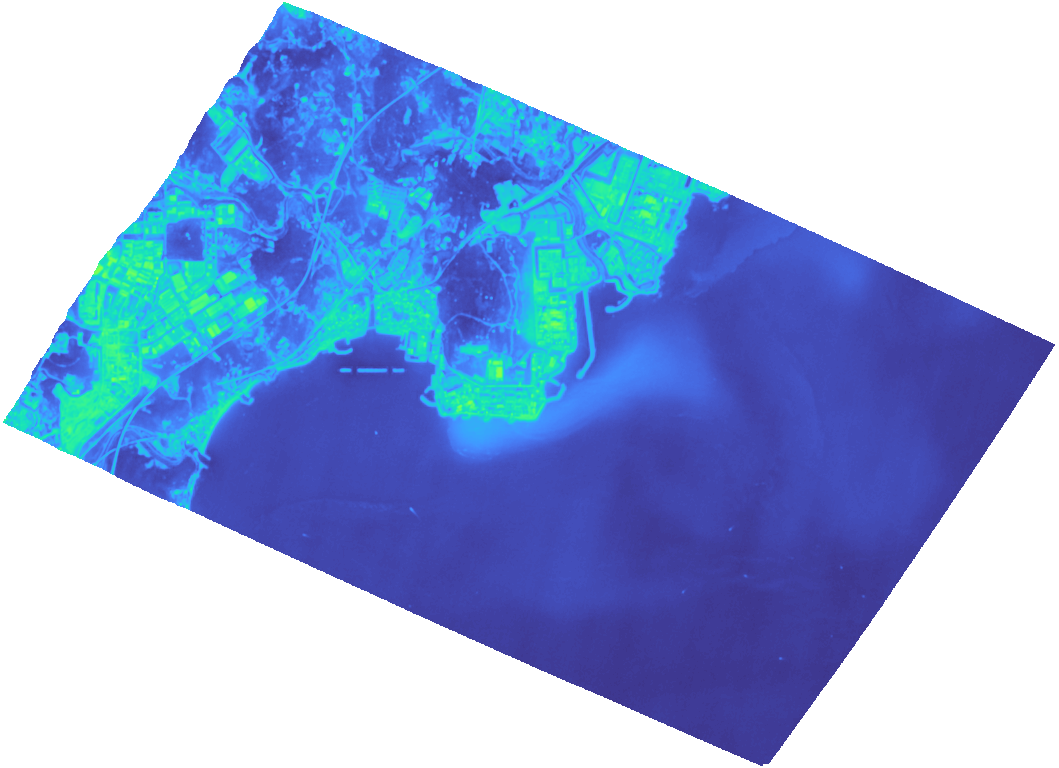
Supplementary Figure A1 · comparison with a shared 20–50°C display range
Image temporarily withheld
 N
N↑2 km
 N
N↑2 km
 N
N↑2 km
Source: comparison_20231016_20231026/visuals/*_10m_Turbo_20-50C.png. The background in this supplementary figure represents no-data areas.