Abstract
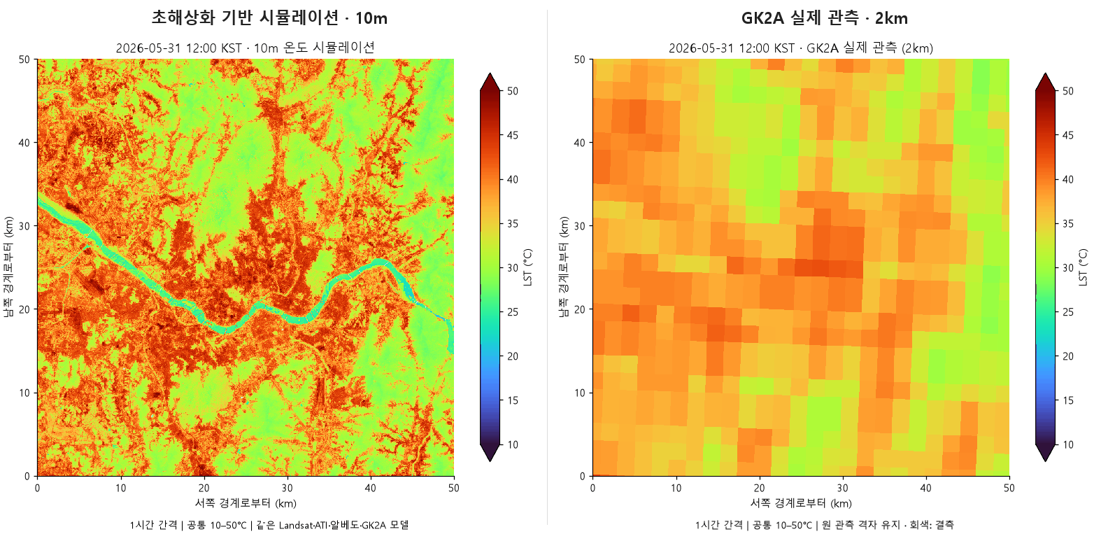
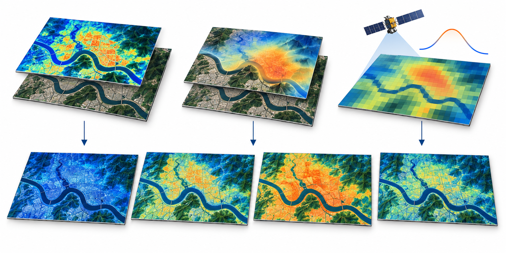
This preliminary experiment reconstructs diurnal land surface temperature (LST) over a 50 × 50 km area of Seoul by combining spatially detailed polar-orbiting satellite data with temporally dense geostationary observations. Its purpose is to explore how far hourly spatial downscaling can be taken. A Landsat-based temperature field downscaled to a 10 m grid at 11:10 Korea Standard Time (KST) on 31 May 2026 provides the spatial reference. Apparent thermal inertia (ATI) and an albedo approximation, derived from day/night temperatures and reflectance from the Visible Infrared Imaging Radiometer Suite (VIIRS), are downscaled using Sentinel-2 optical data. A common temporal curve obtained from 12 GEO-KOMPSAT-2A (GK2A) cells on the same day is combined with pixel-specific amplitudes to generate 25 hourly temperature fields from 00:00 to 00:00 the following day. Each image contains 24,993,576 valid grid cells. Comparisons of native GK2A 2 km cell means at 7 representative times yield root mean square (RMS) differences of 1.42–2.32°C and mean biases of −0.73 to +0.54°C. At 12:00, simulated means are 27.44°C for water, 32.97°C for vegetation and 41.90°C for non-vegetated cover. The experiment is useful in implementing a framework that links spatial information from polar-orbiting satellites with temporal information from a geostationary satellite to explore diurnal changes in the relative thermal environment on a 10 m grid. However, because same-day GK2A and VIIRS night-time information are used in the model, observational consistency comparisons are distinguished from independent validation of 10 m temperature accuracy.
Background and objectives
Understanding the urban thermal environment requires examining both the locations of warmer and cooler areas and their heating and cooling over time. Combining spatial information from polar-orbiting thermal imagery with temporal information from geostationary observations connects these two needs. Earlier work that spatially disaggregates temperature-curve control parameters using optical data provides a methodological basis for this approach.[1]
Using the case of 31 May 2026, this experiment explores the potential of multi-satellite integration and identifies improvements for the next stage. Here, super-resolution refers to empirical spatial downscaling that combines existing temperature and optical information. The central question is whether a high-resolution temperature field at one time, combined with location-specific amplitudes and a geostationary temporal curve, can represent the diurnal thermal environment within a consistent framework.
Data and methods
2.1 Study area and observations
The study covers a 50 × 50 km area of Seoul and its surroundings. In Universal Transverse Mercator (UTM) zone 52N, the west/south/east/north bounds are 299,000 / 4,136,000 / 349,000 / 4,186,000 m. The common model grid contains 5,000 × 5,000 cells at 10 m spacing. Its coordinate reference identifier is European Petroleum Survey Group (EPSG):32652.
| Data | Time (KST) | Role and spatial support |
|---|---|---|
| Landsat 8 | 11:10:07.782370 | Reflectance-matching reference and temperature reference based on the radiative transfer equation (RTE). Reuses the existing 10 m downscaling result |
| Sentinel-2 | 11:15:29 | B02, B03, B04 and B08 at 10 m; B11 at 20 m. Spatial downscaling of optical parameters |
| Suomi-NPP (Suomi National Polar-orbiting Partnership) VIIRS | Approximately 02:55 / 14:16 | VNP21 day/night LST and VNP09 reflectance. 1 km denotes the common alignment grid |
| GK2A Advanced Meteorological Imager (AMI) LST | 00:00–00:00 the following day | Native Korea (KO) domain, 2 km Lambert Conformal Conic (LCC) grid. Data used at 10-minute intervals; 25 hourly outputs |
Of 145 nominal GK2A timestamps, 144 files were available; only 00:20 is missing. All 25 hourly files are present. This collection interval should not be equated with the sensor's entire native observation schedule. The GK2A product estimates land surface temperature using surface emissivity and infrared-channel information.[2] Native VIIRS swath observation times and centre locations were tracked, and the 12:36 scene with a large viewing angle had been excluded in the original experiment.
2.2 Inter-sensor reflectance matching and optical ATI
VIIRS and Sentinel blue, green, red, near-infrared (NIR) and short-wave infrared 1 (SWIR1) reflectance were regression-adjusted to Landsat-equivalent values. VIIRS M3, M4, M5, M7 and M10 were paired with Landsat B2, B3, B4, B5 and B6, respectively. Bandwise linear regressions used 2,643 samples, each comprising one matching Landsat mean per native VIIRS centre. Sentinel data were area-averaged to the native Landsat 30 m grid. For Sentinel B11, a continuous piecewise regression with a knot at 0.05 was adopted to reduce water-related bias. No forced clipping of input reflectance or additional exclusion of water was applied.
Equation (1) is the piecewise regression applied only to Sentinel-2 B11. Here, x is physical Sentinel B11 reflectance and S is Landsat-equivalent SWIR1. Separate bandwise linear coefficients were used for the VIIRS-to-Landsat transformation described above. This is empirical matching for this scene, not an intrinsic sensor calibration applicable to every date.
The ATI target was constructed from an albedo approximation α9, based on VIIRS 9-band directional reflectance, and the temperature difference at the actual day/night observation times. α9 is distinct from VNP43 bidirectional reflectance distribution function (BRDF)-based albedo and measured albedo. The temperature difference is not the daily maximum-minus-minimum difference.
The constant C=1 and the unit is K−1. The 2,498 valid cells on the 1 km alignment grid were grouped by native daytime VIIRS centre to produce 2,126 training samples. Repeated assignments of the same native observation were not counted as independent samples.
The predictors f comprise blue, green, red, near-infrared and short-wave infrared reflectance [B, G, R, N, S], the normalized difference vegetation index (NDVI), normalized difference moisture index (NDMI) and modified normalized difference water index (MNDWI). Additive ridge regression was applied to log ATI with λ=0.003 and a=−3.12781512602881. Predictor effects are smoothly attenuated farther from the training centre to reduce excessive amplification. Location coordinates and water classification were not used as predictors. Regularization strength was selected using nested 5-fold validation with 10 km spatial blocks, at least 2 km separation between native observation centres in training and validation samples, and exclusion of shared native day/night observations. However, the model form was chosen after inspecting the same-day anomaly in the western Han River, so this is not independent validation after model selection.
2.3 Albedo approximation and Landsat spatial reference
A separate 5-band ridge regression with non-negative slopes (λ=0.001) was trained against the VIIRS 9-band albedo approximation and then applied to Sentinel. It used 2,128 native daytime VIIRS centres. ATI and albedo are separate regression estimates.
+ 0R + 0.30867345N + 0.23192344S(5)
The spatial reference TL reuses the existing Landsat super-resolution result for 31 May 2026. Landsat RTE temperature was regressed on Sentinel NDVI, the normalized difference built-up index (NDBI) and the green–NIR normalized difference water index (NDWI), with 30 m residuals distributed through a smooth bilinear control field. The original temperature regression and reflectance correction were retained, not replaced by the current 5-band correction for ATI. A 5 m offset from the original grid was aligned by weighting each of 4 neighbouring pixels by 0.25. Cloud effects included in the original residual calculation were not completely removed by subsequent masking.
2.4 GK2A common curve and hourly integration
A cubic B-spline with 2-hour knots was fitted to diurnal observations from 12 fixed GK2A cells spanning urban, vegetated and water areas. Huber iteratively reweighted least squares (IRLS; 1.5 K) and a second-derivative penalty of λ=0.3 reduced the influence of abrupt changes. After subtracting each curve's 03:00–05:00 mean and normalizing by its difference from the 09:00–16:00 maximum, the pointwise median of the 12 normalized curves was sampled at 5-minute intervals and fitted by least squares using the same spline basis. It was then renormalized to a 03:00–05:00 mean of 0 and a 09:00–16:00 maximum of 1 and fixed as the common curve g(t). This is fitting-weight adjustment to reduce outlier influence, not an observation-removal mask.
Here, tL=11.1688284361 h and g(tL)=0.8699051530. The times td and tn are the actual observation times of the native VIIRS cells. Thus, T(x,tL)=TL(x). The 25 hourly temperatures were generated by directly evaluating the fixed spline at each time, not by interpolating between the existing images at 4-hour intervals. The values g(0)=0.07633523 and g(24)=−0.19163765 are distinct; no extrapolation beyond 0–24 h or periodic connection was applied.
2.5 Quality information and evaluation definitions
Actual missing/fill values and the existing criteria for excluding certain clouds were retained. Water, shadows, cirrus, saturation and out-of-range values were preserved with the original quality assurance (QA) information; missing values were not filled from neighbours. The final common-valid grid contains 24,993,576 valid and 6,424 missing cells. The 248 pixels with negative temperature-amplitude coefficients caused by albedo approximations exceeding 1 were retained and recorded in QA rather than deleted. Their temperatures vary in the opposite direction to the common temporal curve, so they remain a priority for further checks.
Comparisons used native GK2A KO 2 km cells fully contained within the study area. Each 10 m pixel centre was transformed to the KO coordinate system and assigned once to a single cell; equal-area valid pixels were then averaged. This was not a simple comparison between aligned 2 km UTM images. At the 7 representative times, the number of common cells ranges from 518 to 539, with 518 cells common to all 7 times.
Experimental results
3.1 Reproduction of optical parameters
| Target | Native-centre samples | RMSE | R² |
|---|---|---|---|
| Optical ATI · all | 2,126 | 0.00569 K⁻¹ | 0.78715 |
| Optical ATI · water/coastal | 173 | 0.01410 K⁻¹ | 0.73370 |
| Albedo approximation · all | 2,128 | 0.000839 | 0.99790 |
Overall optical ATI RMSE was 0.00569 K−1, with R²=0.787. With the stabilized model, the ratio of median ATI in the central versus western Han River decreased from 14.14 to 1.01. The albedo approximation's R²=0.99790 measures how well 5 bands reproduce an already defined 9-band approximation. Neither metric should be extrapolated to the measured accuracy of independent physical properties or high-resolution temperature.
3.2 Spatial temperature fields through the day
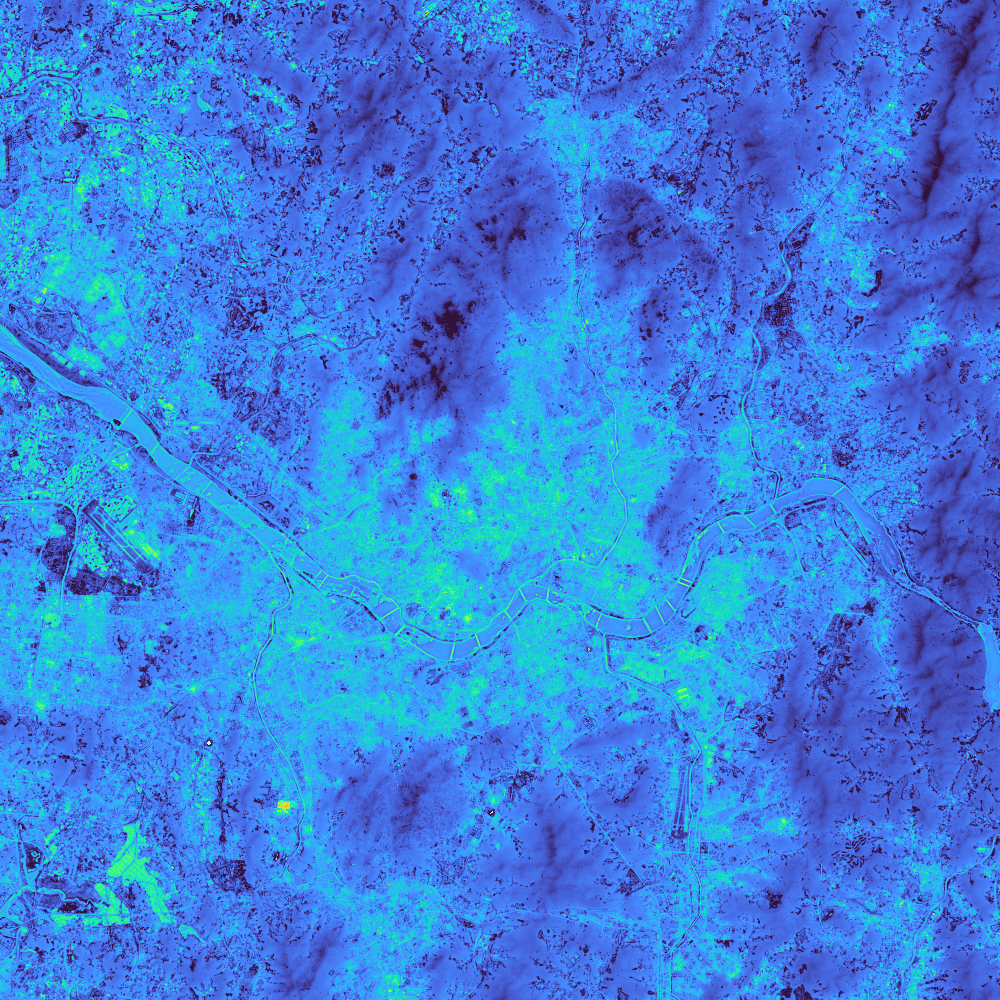
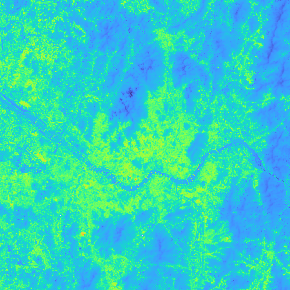
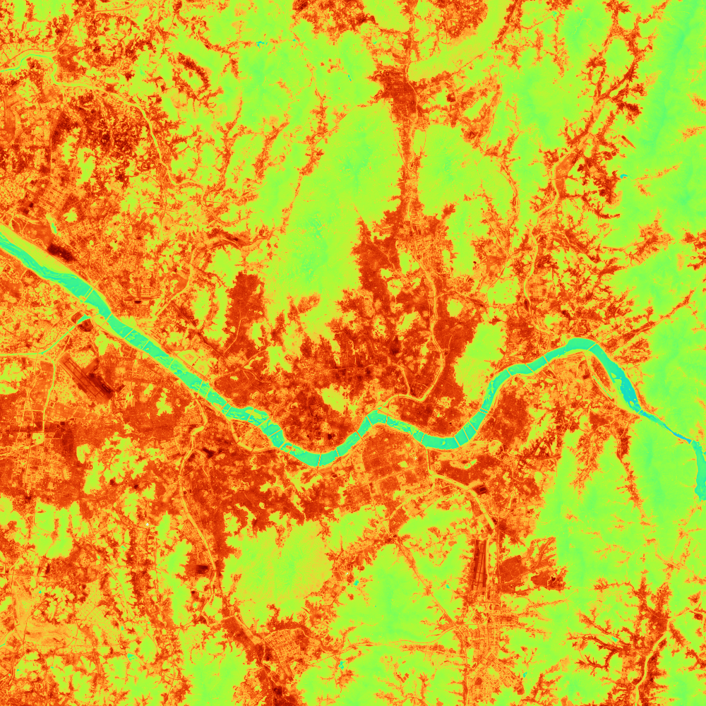
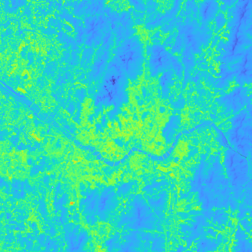
All 25 hourly images, comprising the existing 7 times plus 18 intervening times, retain the same grid and missing-data mask. The whole-area model mean was 16.25°C at 05:00 and 36.97°C at 13:00. Because amplitude varies by location, this is not equivalent to adding or subtracting the same temperature at every pixel.
 N
N↑10 km
 N
N↑10 km
 N
N↑10 km
 N
N↑10 km
Land-cover means were grouped into water, vegetation and non-vegetated cover using the Sentinel-2 Scene Classification Layer (SCL).
At 04:00, water and non-vegetated means were 18.95°C and 18.17°C, respectively; at 12:00, they were 27.44°C and 41.90°C, changing both their ordering and contrast. This results from location-specific amplitudes determined by optical ATI and albedo. The water temperature peak is not separately delayed: except for the exceptional pixels with negative temperature-amplitude coefficients, all locations share the common curve's peak time.
3.3 Consistency with native GK2A observations
| KST | Common cells | Model °C | GK2A °C | Bias °C | RMS °C |
|---|---|---|---|---|---|
| 00:00 | 539 | 18.16 | 17.96 | +0.21 | 1.57 |
| 04:00 | 539 | 16.59 | 16.20 | +0.39 | 1.47 |
| 08:00 | 539 | 22.38 | 22.40 | -0.02 | 1.42 |
| 12:00 | 539 | 36.25 | 36.05 | +0.19 | 2.07 |
| 16:00 | 539 | 32.15 | 32.28 | -0.14 | 2.24 |
| 20:00 | 539 | 22.48 | 21.93 | +0.54 | 1.79 |
| 00:00 next day | 518 | 12.67 | 13.40 | -0.73 | 2.32 |
Values use the common-valid cells at each time. Model means in Table 3 weight the 2 km cells equally and therefore differ from whole-area means of 10 m pixels. Existing comparison results were used without additional fitting of data, coefficients or bias corrections.
Across the 7 times, mean bias was relatively small at −0.73 to +0.54°C, while RMS differences for individual 2 km cells were 1.42–2.32°C. Agreement in spatial means and cellwise differences provide different information. Because the same GK2A data were used to construct the temporal curve, this range is not presented as independent prediction error.
3.4 Hourly comparison and numerical reproducibility
The representative result (Figure 5) allows playback and comparison of hourly changes in the model and GK2A observations from 00:00 to 00:00 the following day.
The original verification compared 25 times × 25 million pixels against the input equations and found a maximum difference of 0.00000191°C. Pixels and files for the existing 7 images at 4-hour intervals were retained, and the band order, timestamps and missing-data masks in the Virtual Raster (VRT) were verified. VRT connects source images as a virtual raster by referencing file paths and band configurations without duplicating the images (official format documentation). This demonstrates computational and storage reproducibility, not accuracy relative to observed temperatures.
Discussion and limitations
4.1 Value for detailed exploration of the diurnal thermal environment
Separating the spatial reference TL from location-specific amplitude A allows more varied relative temperature changes than shifting a single temperature map through the day with unchanged contrast. The water, vegetation and non-vegetated means in this experiment demonstrate that implementation. It can help explore areas that become relatively warmer or cooler over time and select locations and times for additional field observations.
4.2 Common temporal shape and data dependencies
Because all pixels share the same g(t), the model does not separately represent land-cover-specific peak delays, phase differences due to water heat storage, or local weather changes. The optical ATI training target includes VIIRS night-time temperature from the same date. Not directly reading night-time LST during final temperature generation does not make this a prediction made without night-time information. GK2A is also used both for the temporal curve and for comparison, requiring independent evaluation with held-out dates and times.
4.3 Physical meaning of ATI, albedo and 10 m temperature
ATI is an apparent index that depends on observation time, reflectance and the day/night temperature difference, not a direct measurement of physical thermal inertia or soil moisture. The directional-reflectance-based albedo approximation is likewise distinct from independent albedo. Estimating thermal-variation parameters from same-day optical data incorporates empirical relationships among cover types and the influence of spectral indices. High explanatory power in a single-scene regression cannot be interpreted as physical universality across seasons.
The 10 m value denotes output grid spacing. Constraints remain from Landsat thermal information, the native 20 m detail of Sentinel B11, and each sensor's point spread function (PSF), viewing angle and spatial mixing. Many fine-scale temperature fields can produce the same 2 km average. Agreement with GK2A alone therefore cannot validate fine hotspots or absolute 10 m temperatures of individual facilities.
4.4 Missing data and the day boundary
Abrupt late-night drops or spatial changes in native GK2A data may include effects of residual clouds, retrieval errors and changing samples. A data quality flag (DQF)=0 does not establish every abrupt change as a real surface change. The starting midnight and the following midnight represent different observational states and have different values; however, a non-periodic curve for one date cannot be repeated throughout the year. The 248 negative-amplitude pixels and cloud effects in the original Landsat residuals require further QA and model refinement.
Conclusions and next steps
The experiment is useful in implementing a framework that links spatial information from polar-orbiting satellites with temporal information from a geostationary satellite to explore diurnal changes in the relative thermal environment on a 10 m grid. The 25 hourly images, changing land-cover contrasts and relatively small mean biases in native GK2A cells support further investigation. These are therefore preliminary results demonstrating the feasibility of diurnal spatial downscaling. Their current value lies in exploring relative thermal changes and formulating hypotheses and follow-up experiments for validation with independent observations.
The central next step is to test whether hourly thermal-environment structure is maintained on different dates and in different seasons. The extensions proposed in the source document can be summarized as follows.
Research on year-round temperature production combining geostationary and polar-orbiting observations with reanalysis and radiation data provides context for such operational extensions.[3] It does not validate the 10 m performance of this case. The items above summarize follow-up proposals in the source document; no new implementation or performance results were added in this note.
References
- Zhan, W., Huang, F., Quan, J., Zhu, X., Gao, L., Zhou, J., & Ju, W. (2016). Disaggregation of remotely sensed land surface temperature: A new dynamic methodology. Journal of Geophysical Research: Atmospheres, 121, 10538–10554. 10.1002/2016JD024891. Methodological background for downscaling using temporal-curve parameters.
- Korea Meteorological Administration, National Meteorological Satellite Center. GK2A product definitions — land surface temperature (LST). Official product description. Accessed 8 October 2026. Actual timestamps, grids and QA follow the source-data records for this experiment.
- Jia, A., et al. (2023). Global hourly, 5 km, all-sky land surface temperature data from 2011 to 2021 based on integrating geostationary and polar-orbiting satellite data. Earth System Science Data, 15, 869–895. 10.5194/essd-15-869-2023. Background for year-round production, not evidence of this model's performance.
Supplementary material
Appendix A · Optical ATI coefficients and exact reproducibility records
Coefficients in the table are rounded for display. Exact reproduction uses coefficients, normalization constants and the spline in separately stored JavaScript Object Notation (JSON) files. Here f=[B,G,R,N,S,NDVI,NDMI,MNDWI], with NDVI=(N−R)/(N+R), NDMI=(N−S)/(N+S) and MNDWI=(G−S)/(G+S).
| Predictor | μ | σ | β |
|---|---|---|---|
| B | 0.05193822 | 0.02060233 | +0.11559502 |
| G | 0.07949551 | 0.02492671 | -0.06628613 |
| R | 0.07372605 | 0.03278281 | -0.30720673 |
| N | 0.29918487 | 0.06782785 | +0.05304051 |
| S | 0.18356505 | 0.02769897 | -0.07024577 |
| NDVI | 0.58703627 | 0.20540090 | -0.42157552 |
| NDMI | 0.22977259 | 0.11414387 | +0.22961908 |
| MNDWI | -0.40243778 | 0.14009244 | -0.05965599 |